https://blog.csdn.net/program_developer/article/details/80632779的补充
PCA的理论推导
PCA有两种通俗易懂的解释:(1)最小化降维造成的损失;(2)最大方差理论。这两个思路都能推导出同样的结果。
reconstruction error
Find vectors in a subspace that are closest to data points.
$\min_{U} \frac{1}{N} \sum_{i=1}^{N}\left|\mathbf{x}^{(i)}-\tilde{\mathbf{x}}^{(i)}\right|^{2}$
variance of reconstructions
Find a subspace where data has the most variability.
$\max_{U} \frac{1}{N} \sum_{i}\left|\tilde{\mathbf{x}}^{(i)}-\hat{\boldsymbol{\mu}}\right|^{2}$
We show that
$$
\frac{1}{N} \sum_{i=1}^{N}\left|\mathbf{x}^{(i)}-\tilde{\mathbf{x}}^{(i)}\right|^{2}=\text { const }-\frac{1}{N} \sum_{i}\left|\tilde{\mathbf{x}}^{(i)}-\hat{\boldsymbol{\mu}}\right|^{2}
$$
$\textbf{ Observation 1}$: As $|\mathbf{v}|^{2}=\mathbf{v}^{\top} \mathbf{v}$ and $\mathbf{U}^{\top} \mathbf{U}=I,$ we have
$|\mathbf{U} \mathbf{v}|^{2}=\mathbf{v}^{\top} \mathbf{U}^{\top} \mathbf{U} \mathbf{v}=|v|^{2} .$ Therefore
$\left|\tilde{\mathbf{x}}^{(i)}-\hat{\boldsymbol{\mu}}\right|^{2}=\left(\mathbf{U} \mathbf{z}^{(i)}\right)^{\top}\left(\mathbf{U} \mathbf{z}^{(i)}\right)=\left[z^{(i)}\right]^{\top} \mathbf{U}^{\top} \mathbf{U} \mathbf{z}^{(i)}=\left[z^{(i)}\right]^{\top} \mathbf{z}^{(i)}=\left|\mathbf{z}^{(i)}\right|^{2}$
$\textbf{ Observation 2:}$
To show the orthogonality of $\tilde{\mathbf{x}}^{(i)}-\hat{\boldsymbol{\mu}}$ and $\tilde{\mathbf{x}}^{(i)}-\mathbf{x}^{(i)},$ observe that
$\left(\tilde{\mathbf{x}}^{(i)}-\hat{\boldsymbol{\mu}}\right)^{\top}\left(\tilde{\mathbf{x}}^{(i)}-\mathbf{x}^{(i)}\right)$
$=\left(\mathbf{x}^{(i)}-\hat{\boldsymbol{\mu}}\right) \quad \mathbf{U} \mathbf{U}^{\top}\left(\hat{\boldsymbol{\mu}}-\mathbf{x}^{(i)}+\mathbf{U} \mathbf{U}^{\top}\left(\mathbf{x}^{(i)}-\hat{\boldsymbol{\mu}}\right)\right)$
$=\left(\mathbf{x}^{(i)}-\hat{\boldsymbol{\mu}}\right)^{\top} \mathbf{U} \mathbf{U}^{\top}\left(\hat{\boldsymbol{\mu}}-\mathbf{x}^{(i)}\right)+\left(\mathbf{x}^{(i)}-\hat{\boldsymbol{\mu}}\right)^{\top} \mathbf{U} \mathbf{U}^{\top}\left(\mathbf{x}^{(i)}-\hat{\boldsymbol{\mu}}\right)$
=0
Because of the orthogonality of $\tilde{\mathbf{x}}^{(i)}-\hat{\boldsymbol{\mu}}$ and $\tilde{\mathbf{x}}^{(i)}-\mathbf{x}^{(i)},$ we can use the Pythagorean theorem(勾股定理) to conclude that
$\left|\tilde{\mathbf{x}}^{(i)}-\hat{\boldsymbol{\mu}}\right|^{2}+\left|\mathbf{x}^{(i)}-\tilde{\mathbf{x}}^{(i)}\right|^{2}=\left|\mathbf{x}^{(i)}-\hat{\boldsymbol{\mu}}\right|^{2}$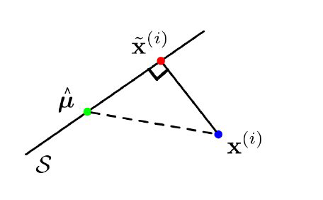
then we have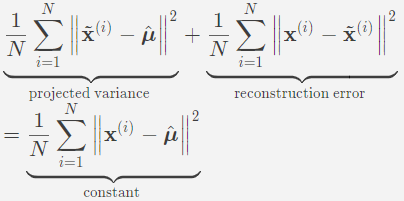
Therefore, projected variance = constant + reconstruction error.Maximizing the variance is equivalent to minimizing the reconstruction error!
找到PCA
For $K=1,$ we are fitting a unit vector $\mathbf{u},$ and the code is a scalar $z^{(i)}=\mathbf{u}^{\top}\left(\mathbf{x}^{(i)}-\hat{\boldsymbol{\mu}}\right) .$ Let’s maximize the projected variance. From Observation 1, we have
$\begin{aligned} \frac{1}{N} \sum_{i}\left|\tilde{\mathbf{x}}^{(i)}-\hat{\boldsymbol{\mu}}\right|^{2} &=\frac{1}{N} \sum_{i}\left|z^{(i)}\right|^{2}=\frac{1}{N} \sum_{i}\left(\mathbf{u}^{\top}\left(\mathbf{x}^{(i)}-\hat{\boldsymbol{\mu}}\right)\right)^{2} \ \end{aligned}$
$=\frac{1}{N} \sum_{i=1}^{N} \mathbf{u}^{\top}\left(\mathbf{x}^{(i)}-\hat{\boldsymbol{\mu}}\right)\left(\mathbf{x}^{(i)}-\hat{\boldsymbol{\mu}}\right)^{\top} \mathbf{u}$
$=\mathbf{u}^{\top}\left[\frac{1}{N} \sum_{i=1}^{N}\left(\mathbf{x}^{(i)}-\hat{\boldsymbol{\mu}}\right)\left(\mathbf{x}^{(i)}-\hat{\boldsymbol{\mu}}\right)^{\top}\right] \mathbf{u}$
$\begin{aligned}
&=\mathbf{u}^{\top} \hat{\mathbf{\Sigma}} \mathbf{u}\
&=\mathbf{u}^{\top} \mathbf{Q} \mathbf{\Lambda} \mathbf{Q}^{\top} \mathbf{u} \text { for } \mathbf{a}=\mathbf{Q}^{\top} \mathbf{u} \
&=\mathbf{a}^{\top} \mathbf{\Lambda} \mathbf{a}\
&=\sum_{j=1}^{D} \lambda_{j} a_{j}^{2}
\end{aligned}$
A similar argument shows that the $k$ th principal component is the $k$ th eigenvector of $\boldsymbol{\Sigma} .$ If you’re interested, look up the Courant-Fischer Theorem.
extra features , Decorralation about features:
Cov (.) denote the empirical covariance.
$\begin{aligned}
\operatorname{Cov}(\mathbf{z}) &=\operatorname{Cov}\left(\mathbf{U}^{\top}(\mathbf{x}-\boldsymbol{\mu})\right) \
&=\mathbf{U}^{\top} \mathbf{C o v}(\mathbf{x}) \mathbf{U} \
&=\mathbf{U}^{\top} \mathbf{\Sigma} \mathbf{U} \
&=\mathbf{U}^{\top} \mathbf{Q} \mathbf{\Lambda} \mathbf{Q}^{\top} \mathbf{U} \
&=(\mathbf{I} \quad \mathbf{0}) \mathbf{\Lambda}\left(\begin{array}{l}
\mathbf{I} \
0
\end{array}\right) \
&=\operatorname{top} \operatorname{left} K \times K \text { block of } \mathbf{\Lambda}
\end{aligned}$
If the covariance matrix is diagonal, this means the features are uncorrelated.
总结
1 Dimensionality reduction aims to find a low-dimensional representation of the data.
2 PCA projects the data onto a subspace which maximizes the projected variance, or equivalently, minimizes the reconstruction error.
3 $\textbf{The optimal subspace is given by the top eigenvectors}$
$\textbf{of the empirical covariance matrix.}$
4 $\textbf{PCA gives a set of decorrelated features.}$
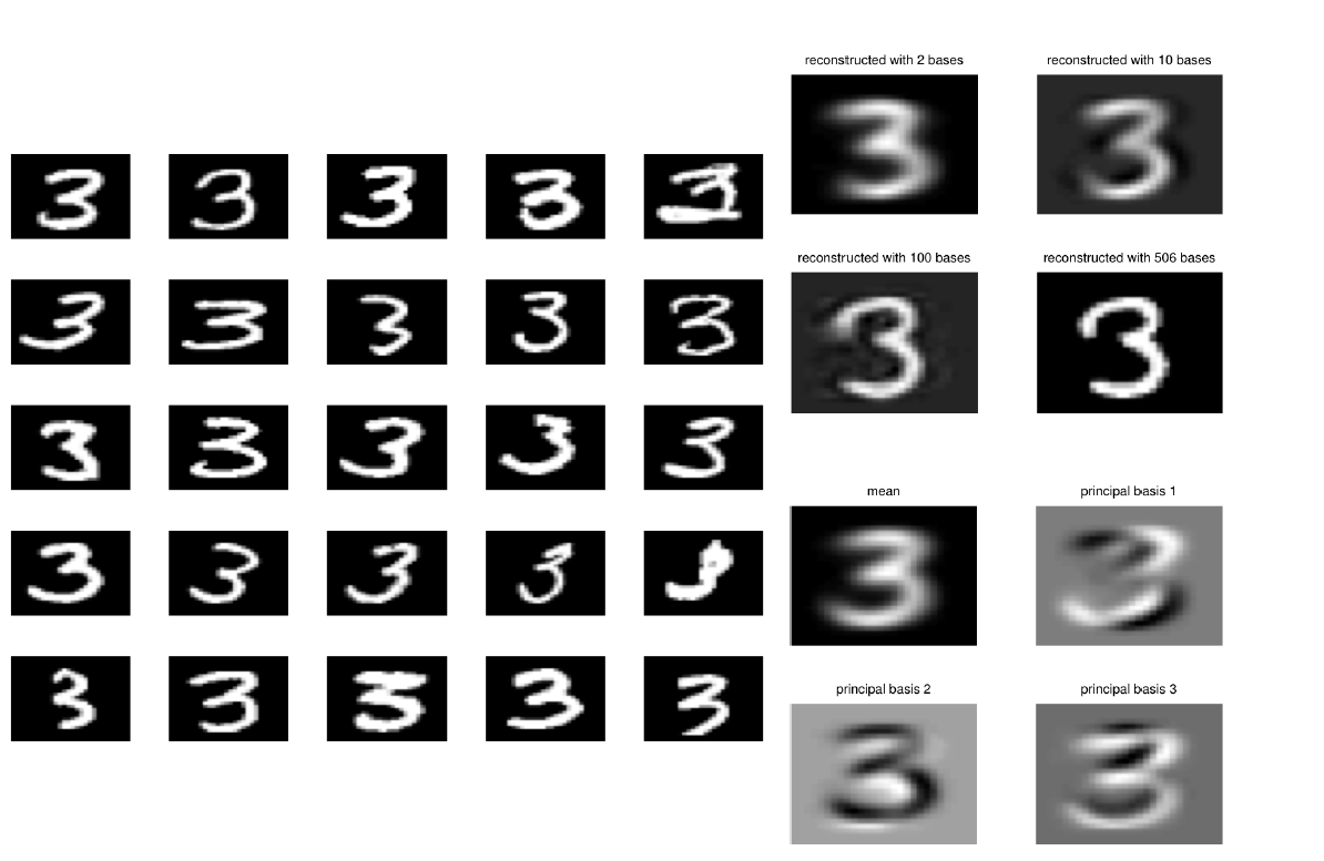
例子